A trading strategy that returned 40% last year sounds better than one that returned 20%. Then you learn the first one swung wildly enough to halve your account twice along the way, and the second barely flinched. Suddenly the raw return tells you almost nothing. The Sharpe ratio exists to settle exactly this kind of comparison: it measures the return a strategy earned against the risk it took to earn it.
Definition
"The Sharpe ratio is a strategy's average return above the risk-free rate divided by the standard deviation of its returns, a measure of return earned per unit of risk."
The measure comes from William Sharpe, who introduced it in 1966 as the reward-to-variability ratio and refined it in a 1994 paper for the Journal of Portfolio Management. In that paper he defined it as the expected differential return per unit of risk associated with that differential return. In plainer terms, the numerator is the return a strategy earns above a benchmark, usually the risk-free rate, the rate you could have earned holding something safe. The denominator is the standard deviation of those returns, a measure of how much they bounce around.
That structure is the whole idea. A strategy is rewarded for return and charged for the jumpiness of getting it. A higher Sharpe ratio means more return per unit of risk taken. This is why a calmer 20% can outrank a chaotic 40%, and why the ratio has become a standard yardstick for comparing strategies, funds, and portfolios that otherwise look incomparable.
It measures the return a strategy earned against the risk it took to earn it.How the Sharpe ratio is built
Three inputs go in, and each one carries an assumption worth knowing.
The first is the strategy's return over a period. The second is the risk-free rate, subtracted from that return to leave the excess, the part you were actually paid for taking risk rather than the part you could have earned safely. The third is the standard deviation of the returns, which stands in for risk. In practice the ratio is built from a series of periodic returns: for each period you take the excess return over the risk-free rate, then divide the average of those excess returns by their standard deviation.
Sharpe Ratio = Average Excess Return ÷ Standard Deviation of Excess Returns

Excess Return = Strategy Return − Risk-Free Rate, measured each period
Standard deviation is doing heavy lifting here, and it is worth pausing on. It treats every deviation from the average the same, whether the return came in far above expectations or far below. A month of unexpected gains widens the standard deviation exactly as much as a month of unexpected losses. The Sharpe ratio, by construction, penalizes upside volatility as if it were a problem, which for most traders it is not.
The Sharpe ratio also depends on the period it is measured over, a detail Sharpe himself stressed. The ratio is not independent of the time period over which it is measured. A figure built from daily returns and one built from monthly returns are not directly comparable, because returns grow with time while volatility grows with the square root of time. Andrew Lo, in a 2002 Financial Analysts Journal paper, showed that monthly Sharpe ratios cannot simply be annualized by multiplying by the square root of twelve except under narrow assumptions. Two Sharpe ratios are only comparable when they were computed the same way, over the same kind of period.
A small worked example makes the formula concrete. Suppose a strategy's monthly numbers look like this.
| Input | Value |
|---|---|
| Average monthly strategy return | 1.5% |
| Monthly risk-free return | 0.5% |
| Average monthly excess return | 1.0% |
| Standard deviation of monthly excess returns | 4.0% |
| Monthly Sharpe ratio | 0.25 |
Illustrative figures.
The strategy earned 0.25 units of excess return for each unit of monthly volatility. Annualised under the usual assumption, this becomes roughly 0.25 × √12 ≈ 0.87, but that step is only valid when the periodic returns are independent and measured consistently, the caveat Andrew Lo raised above.
How to read the number
A Sharpe ratio has no natural ceiling, but it does have a rough reading. As a loose convention, above 1 is often treated as respectable and above 2 as strong, though many practitioners treat anything much higher with suspicion. Below 1, the strategy is delivering modest return for the risk it carries, and a ratio near zero or negative means the excess return did not justify the volatility at all.
| Sharpe ratio | Rough reading | What to do next |
|---|---|---|
| Below 0 | Negative excess return per unit of volatility | Reject, or investigate deeply |
| 0 to 1 | Weak to modest risk-adjusted return | Check drawdown, costs, and consistency |
| 1 to 2 | Respectable if the assumptions are realistic | Compare against similar strategies |
| 2 to 3 | Strong, but inspect for smoothing or cherry-picking | Validate across regimes |
| Above 3 | Exceptional, and suspicious without strong evidence | Check data quality, liquidity, and overfitting |
Those thresholds are a starting point, not a law. The same number means different things for a single volatile instrument and a diversified portfolio, and it shifts with the market regime the returns were drawn from. A Sharpe ratio is most honest as a relative tool, not as an absolute grade: comparing two strategies tested the same way over the same window, the higher one earned its return more efficiently. Used to grade a single strategy in isolation, it is far shakier.
A Sharpe ratio is most honest as a relative tool, not as an absolute grade.Figure 1 shows the intuition. Two equity curves climb to the same ending point, the same average return. One rises in a near-straight line; the other lurches up and down on its way to the same place. The smooth one has the higher Sharpe ratio, because it produced that return with less volatility underneath it. The picture is the whole concept: same destination, different risk to get there.
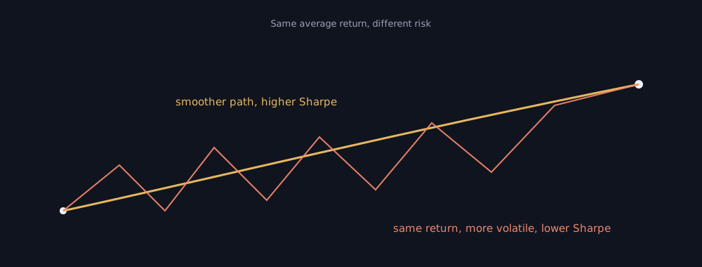
Figure 1: Same average return, different volatility. The smoother path earns the higher Sharpe ratio because it took less risk to reach the same place.
This is also why the ratio matters more for a trader evaluating a backtest than the headline return does. A strategy that looks brilliant on total return can hide a punishing ride, and the depth of that ride is what a maximum drawdown figure and the Sharpe ratio together start to reveal.
The same point falls out of a few numbers. Three strategies, three different trade-offs:
| Strategy | Annual return | Volatility | Sharpe reading |
|---|---|---|---|
| A | 30% | 35% | High return, unstable path |
| B | 22% | 12% | Lower return, better risk-adjusted result |
| C | 18% | 30% | Weak reward for the risk taken |
Illustrative figures, not a real strategy or a recommendation.
On headline return, A wins. On return earned per unit of risk, B wins clearly, and Figure 2 shows why: the steeper the line from the origin, the more return a strategy earned for the volatility it carried. The best strategy is not automatically the one with the highest return; it is the one that gives the best return relative to the risk required to earn it.
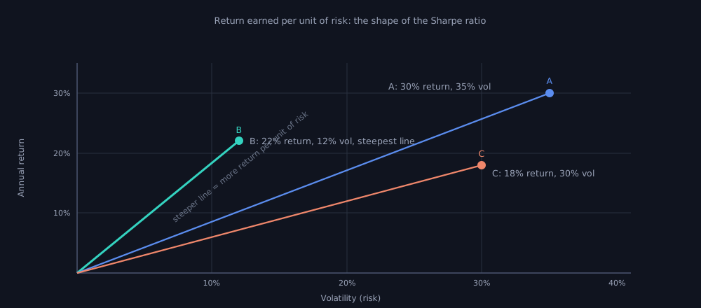
Figure 2: Return earned per unit of risk. Each line runs from the origin to a strategy's return-and-volatility point, and the steeper the line, the higher the reward for the risk taken. B earns the most return for its volatility, even though A has the higher raw return.
Where the Sharpe ratio misleads
The number is only as trustworthy as the returns fed into it, and several things distort it without showing it.
The first is the shape of the returns. The Sharpe ratio is most informative when returns are reasonably well-behaved; it becomes less reliable when returns are highly skewed or fat-tailed, and real strategy returns often are. The CFA Institute notes that asset and factor returns are frequently negatively skewed and show excess kurtosis, or fat tails, meaning extreme moves happen more often than a normal curve predicts. A strategy that sells options, for instance, can show a flattering Sharpe ratio for years while carrying the hidden risk of a rare, severe loss the standard deviation never captured.
Smoothing distorts the number too. When a strategy holds illiquid positions that are marked infrequently, its reported returns look calmer than the underlying reality, which understates volatility and inflates the ratio. Mila Getmansky, Andrew Lo, and Igor Makarov documented this in a 2003 study, finding that smoothed returns from illiquid holdings understate true volatility and raise risk-adjusted measures like the Sharpe ratio. Lo's earlier work put a number on the related effect from serial correlation, the tendency for one period's return to predict the next: an annual Sharpe ratio could be overstated by as much as 65% once that correlation was accounted for.
The number is only as trustworthy as the returns fed into it.Then there is the window. Because the ratio depends on the period it is measured over, a tester can, knowingly or not, pick the stretch of history where a strategy looked best. A Sharpe ratio computed on a hand-picked calm market is not the same number you would get across a full cycle that included a crash. This is the same hazard any backtest carries, and it is one reason a disciplined approach to strategy validation treats a single flattering figure with suspicion rather than trust.
For the specific blind spot of punishing good volatility, there is a direct alternative. The Sortino ratio, developed by Frank Sortino and Lee Price, keeps the same structure but swaps the denominator: instead of total standard deviation, it uses downside deviation, the volatility of returns that fall below a target the trader sets, often called the minimum acceptable return. By penalizing only the returns that fall below that target, the Sortino ratio stops charging a strategy for its upside surprises and focuses on the losses that actually hurt. For a strategy with lopsided returns, frequent small gains and rare large drops, or the reverse, the two ratios can tell noticeably different stories.
Reading it as one signal among several
The Sharpe ratio ranks; it does not grade. It compresses a strategy's whole risk-and-return profile into one number. That makes it easy to rank and easy to over-trust. The compression is useful for ranking, and dangerous if the number is read as a final grade.
Used well, it sits alongside other measures rather than replacing them. The Sortino ratio refines its view of risk; a drawdown figure shows the worst stretch a trader would have had to sit through; the assumptions behind the inputs, the period, the liquidity of the holdings, the shape of the return distribution, decide whether the number can be trusted at all. A Sharpe ratio of 2 on a clean, full-cycle, liquid backtest means something quite different from a 2 squeezed out of a smoothed, cherry-picked window.
A higher Sharpe ratio means more return per unit of risk taken.Treating a metric as a prompt to investigate, not a conclusion, is what a disciplined approach to systematic trading depends on. The number is a prompt to ask what produced it, not a license to stop asking.
A checklist before you trust a Sharpe ratio
Before trusting a Sharpe ratio, ask:
- Was it calculated from daily, weekly, or monthly returns?
- Was it annualised correctly?
- Were the returns liquid and marked honestly?
- Are there signs of serial correlation or smoothing?
- Does the strategy carry fat-tail or crash risk?
- Is the result measured over a full market cycle?
- Does the drawdown tell the same story?
- Does the Sortino ratio confirm or contradict it?
A trading idea earns its Sharpe ratio only inside a test, and the test is where the assumptions either hold or fail silently. Computing the ratio honestly, over a full cycle, on realistic returns, and then reading it next to drawdown and downside risk rather than alone, is part of putting validation between a trading idea and live capital. That is the layer daZh by Zudora is built to be: a place to test an idea against history, inspect the risk-adjusted numbers it produces, and understand what a figure like the Sharpe ratio can and cannot tell you before any money is at stake. A metric cannot promise the next trade. Reading it well means asking what produced the number before trusting it.
Related concepts
- Drawdown, the companion risk metric that captures the worst peak-to-trough fall.
- Strategy validation, the process where risk-adjusted metrics like this one are read.
- How to Choose an Algo Trading Platform.
Disclaimer: daZh is a software platform for building, testing, and managing user-defined trading strategies. It does not provide investment advice, stock recommendations, guaranteed returns, or profit assurance. Backtests are based on historical data and assumptions; actual trading results may differ.
Sources
- William F. Sharpe, "The Sharpe Ratio", The Journal of Portfolio Management, Fall 1994, 21(1): 49 to 58 (author's text). https://web.stanford.edu/~wfsharpe/art/sr/sr.htm
- Andrew W. Lo, "The Statistics of Sharpe Ratios", Financial Analysts Journal, 2002, 58(4): 36 to 52. https://rpc.cfainstitute.org/research/financial-analysts-journal/2002/the-statistics-of-sharpe-ratios
- Mila Getmansky, Andrew W. Lo, Igor Makarov, "An Econometric Model of Serial Correlation and Illiquidity in Hedge Fund Returns", NBER Working Paper 9571, 2003. https://www.nber.org/papers/w9571
- CFA Institute, "Backtesting and Simulation", CFA Program refresher reading, 2026 curriculum. https://www.cfainstitute.org/insights/professional-learning/refresher-readings/2026/backtesting-and-simulation
- Frank A. Sortino and Lee N. Price, "Performance Measurement in a Downside Risk Framework", The Journal of Investing, Fall 1994, 3(3): 59 to 64. DOI: 10.3905/joi.3.3.59. https://joi.iijournals.com/content/3/3/59